Machine Learning Algorithms, Logistic Regression

vdrsoftwareonline.com – Logistic Regression is one of the most fundamental and widely used algorithms in machine learning, especially when dealing with classification problems. Despite its name, logistic regression is not a regression algorithm but rather a classification technique used to predict categorical outcomes. This article will explore what logistic regression is, how it works, its mathematical foundation, how to implement it, and its advantages and limitations.

What is Logistic Regression?

Logistic Regression is a supervised machine learning algorithm used for binary classification tasks—those that involve predicting one of two possible outcomes. It’s commonly used when the dependent variable is categorical, such as “Yes” or “No”, “True” or “False”, “Spam” or “Not Spam”, etc. The goal of logistic regression is to model the probability that a given input belongs to a particular class.

Although it’s called “regression,” logistic regression is used for classification because it predicts probabilities, not continuous values.

How Does Logistic Regression Work?

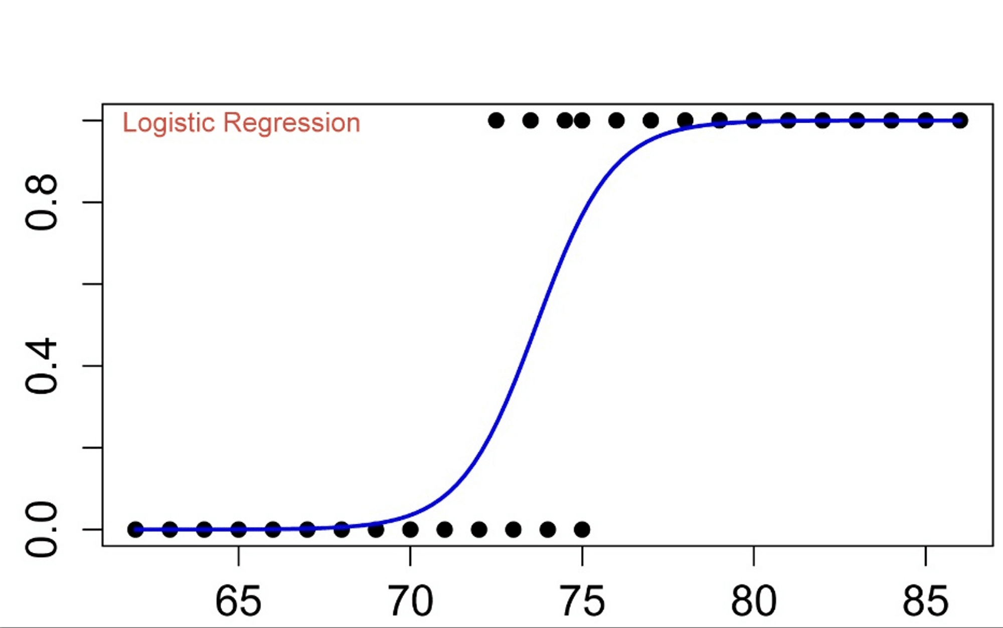
The key idea behind logistic regression is to find the relationship between the dependent variable and the independent variables using a linear function, and then map the result to a probability value between 0 and 1 using the logistic function (also known as the sigmoid function).

1. Linear Combination of Input Features

In logistic regression, the first step is to compute a linear combination of the input features:

z=β0+β1×1+β2×2+⋯+βnxnz = \beta_0 + \beta_1 x_1 + \beta_2 x_2 + \dots + \beta_n x_nz=β0​+β1​x1​+β2​x2​+⋯+βn​xn​

Where:

• $z$ is the linear combination of the input features.
• β0\beta_0β0​ is the intercept (or bias term).
• β1,β2,…,βn\beta_1, \beta_2, \dots, \beta_nβ1​,β2​,…,βn​ are the weights associated with each feature x1,x2,…,xnx_1, x_2, \dots, x_nx1​,x2​,…,xn​.

This equation produces a value for $z$, but it can be any real number, and we want to convert it to a probability between 0 and 1. This is where the sigmoid function comes in.

2. The Sigmoid (Logistic) Function

The sigmoid function is used to squish the output of the linear equation $z$ into a probability:

σ(z)=11+e−z\sigma(z) = \frac{1}{1 + e^{-z}}σ(z)=1+e−z1​

The sigmoid function has the following properties:

• If $z\to \infty$, then $\sigma (z)\to 1$.
• If $z\to -\infty$, then $\sigma (z)\to 0$.
• If $z=0$, then $\sigma (z)=0.5$.

So, for a given set of features x1,x2,…,xnx_1, x_2, \dots, x_nx1​,x2​,…,xn​, the logistic regression model outputs a probability $p$ that the observation belongs to the positive class (class 1). This probability is between 0 and 1, and it can be interpreted as the model’s confidence in classifying the observation as class 1.

3. Decision Threshold

Once the model predicts the probability, we need to decide how to classify the input. A common threshold is 0.5:

• If $\sigma (z)\ge 0.5$, classify the observation as class 1 (positive class).
• If $\sigma (z)<0.5$, classify the observation as class 0 (negative class).

This threshold can be adjusted depending on the application, especially if the costs of false positives and false negatives are not equal.

Cost Function (Binary Cross-Entropy Loss)

The goal of logistic regression is to find the optimal values for the coefficients (weights) β0,β1,…,βn\beta_0, \beta_1, \dots, \beta_nβ0​,β1​,…,βn​ that minimize the difference between the predicted probabilities and the actual labels in the training data. This is done using a cost function.

The cost function used in logistic regression is binary cross-entropy loss (also called log loss). The formula for the binary cross-entropy loss for a single training example is:

J(β)=−[ylog⁡(hβ(x))+(1−y)log⁡(1−hβ(x))]J(\beta) = – \left[ y \log(h_\beta(x)) + (1 – y) \log(1 – h_\beta(x)) \right]J(β)=−[ylog(hβ​(x))+(1−y)log(1−hβ​(x))]

Where:

• $y$ is the actual label (0 or 1),
• hβ(x)h_\beta(x)hβ​(x) is the predicted probability that the example belongs to class 1, given the input features $x$.

The total cost is averaged over all training examples:

J(β)=−1m∑i=1m[y(i)log⁡(hβ(x(i)))+(1−y(i))log⁡(1−hβ(x(i)))]J(\beta) = -\frac{1}{m} \sum_{i=1}^{m} \left[ y^{(i)} \log(h_\beta(x^{(i)})) + (1 – y^{(i)}) \log(1 – h_\beta(x^{(i)})) \right]J(β)=−m1​i=1∑m​[y(i)log(hβ​(x(i)))+(1−y(i))log(1−hβ​(x(i)))]

Where $m$ is the number of training examples.

Optimization: Gradient Descent

To minimize the cost function, logistic regression uses gradient descent, an optimization algorithm. The idea is to iteratively adjust the coefficients $\beta$ in the direction that reduces the cost function.

The gradient descent update rule for each coefficient is:

βj=βj−α⋅∂J(β)∂βj\beta_j = \beta_j – \alpha \cdot \frac{\partial J(\beta)}{\partial \beta_j}βj​=βj​−α⋅∂βj​∂J(β)​

Where:

• $\alpha$ is the learning rate, which controls the size of the step in the gradient descent.
• ∂J(β)∂βj\frac{\partial J(\beta)}{\partial \beta_j}∂βj​∂J(β)​ is the derivative of the cost function with respect to the coefficient βj\beta_jβj​.

Gradient descent continues until the cost function converges to a minimum.

Advantages of Logistic Regression

1. Simplicity and Interpretability: Logistic regression is easy to understand and implement. The coefficients ($\beta$) directly represent the relationship between the features and the outcome, making the model interpretable.
2. Efficiency: It is computationally inexpensive, especially for smaller datasets, and can handle large datasets efficiently with proper regularization.
3. Probabilistic Output: Logistic regression outputs probabilities, which are valuable for decision-making processes. For example, it can be used to estimate the risk of an event happening.
4. Works Well for Linearly Separable Data: Logistic regression performs well when the classes are linearly separable, meaning a straight line or hyperplane can separate the classes.
5. Regularization: Logistic regression can be easily regularized (e.g., using L1 or L2 regularization), which helps prevent overfitting, especially when dealing with high-dimensional data.

Limitations of Logistic Regression

1. Linear Decision Boundary: Logistic regression is limited to problems where the classes are linearly separable or can be separated by a hyperplane. It may not perform well with more complex, non-linear relationships.
2. Sensitive to Outliers: Logistic regression can be sensitive to outliers, which can distort the model’s coefficients and predictions.
3. Requires Feature Engineering: If the relationship between features and the target variable is complex, logistic regression may not capture it unless proper feature engineering is applied.
4. Assumption of Linearity: Logistic regression assumes that the log-odds of the outcome is a linear combination of the input features. If this assumption is violated, the model’s performance may degrade.

Applications of Logistic Regression

Logistic regression is widely used in various fields for classification tasks, including:

1. Healthcare: Predicting the likelihood of a patient having a disease based on diagnostic information (e.g., predicting whether a person has cancer based on medical records).
2. Marketing: Predicting whether a customer will buy a product based on demographic and behavioral data.
3. Finance: Credit scoring models to predict whether a customer will default on a loan.
4. E-commerce: Predicting whether a user will click on an ad or make a purchase.
5. Social Media: Classifying whether a social media post is spam or not.

Conclusion

Logistic Regression remains one of the most popular and effective algorithms for binary classification problems due to its simplicity, interpretability, and probabilistic output. While it may have limitations in handling complex, non-linear relationships or multi-class problems, its ability to produce easily interpretable models and its effectiveness with linearly separable data make it a valuable tool for many machine learning tasks. When implementing logistic regression, it’s crucial to understand its assumptions, advantages, and limitations to ensure it is applied to the right type of problem.